Classification of Flowers In Mobile Phone ( PART 2)

Hey, welcome back! 👋

If you missed Part 1, we loaded the flowers dataset and wrangled it into a clean tf.data pipeline ready to be fed into a model. Go check that out first — this post picks up right where we left off.

Here's the plan for today:

• Build a simple baseline CNN with Keras
• Train it and watch it overfit (classic)
• Fix the overfitting using data augmentation and dropout
• Run inference on a sunflower image
• Convert the model to .tflite for mobile deployment

And in Part 3, we'll build the actual Flutter app that runs this model on-device. Yes, on your phone. Pretty wild, right? Let's get into it.

---

The Baseline Model

We're starting simple. Our first model has three convolution blocks followed by a fully connected layer. Nothing fancy — just enough to get something running so we can see what breaks.

import numpy as np
import tensorflow as tf
from tensorflow import keras
from tensorflow.keras import layers
from tensorflow.keras.models import Sequential

num_classes = len(class_names)

model = Sequential([
    layers.Rescaling(1./255, input_shape=(img_height, img_width, 3)),
    layers.Conv2D(16, 3, padding='same', activation='relu'),
    layers.MaxPooling2D(),
    layers.Conv2D(32, 3, padding='same', activation='relu'),
    layers.MaxPooling2D(),
    layers.Conv2D(64, 3, padding='same', activation='relu'),
    layers.MaxPooling2D(),
    layers.Flatten(),
    layers.Dense(128, activation='relu'),
    layers.Dense(num_classes)
])

Let me walk you through what's happening here, layer by layer.

Rescaling(1./255) — Pixel values in an image go from 0 to 255. We squish them down to [0, 1] so the numbers are well-behaved for training. Always do this.

Conv2D layers — Each of these scans the image with small 3×3 filters, learning to detect features like edges, textures, and shapes. The first one uses 16 filters, and we double that in each subsequent block (16 → 32 → 64). padding='same' means the output keeps the same height/width as the input, so we don't lose edge information.

MaxPooling2D — After each convolution, we downsample the feature maps by 2×2. This shrinks the spatial dimensions, reduces computation, and helps the model focus on dominant features rather than exact pixel positions.

Flatten — At this point the data is a 3D tensor (height × width × channels). The Dense layer downstream needs a flat 1D vector, so this just reshapes it.

Dense(128, activation='relu') — A fully connected layer that combines all the extracted features to learn high-level patterns.

Dense(num_classes) — The output layer. No activation here because we're using from_logits=True in our loss function — meaning we pass raw scores (logits) directly to the loss, and it handles the softmax internally. This is actually numerically more stable.

---

Compiling the Model

model.compile(
    optimizer='adam',
    loss=tf.keras.losses.SparseCategoricalCrossentropy(from_logits=True),
    metrics=['accuracy']
)

Three things happening here:

Optimizer (adam) — This is the algorithm that updates the model's weights after each batch to reduce the loss. Adam is a great default. It adapts the learning rate per parameter, which tends to work well without a lot of tuning.

Loss function (SparseCategoricalCrossentropy) — This measures how wrong the model's predictions are. "Sparse" means our labels are integers (like 0, 1, 2...) rather than one-hot encoded vectors. from_logits=True tells the loss that we're feeding it raw logits, not probabilities.

Metrics (accuracy) — Just tells Keras to also report accuracy during training. It doesn't affect training itself, it's just for us to monitor progress.

You can peek at the full architecture and parameter count like this:

model.summary()

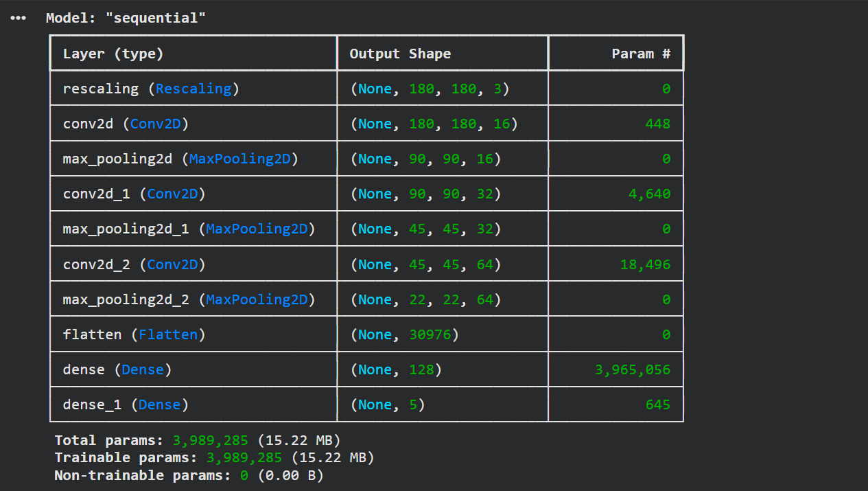Model summary showing ~4 million parameters

About 4 million parameters — that's 4 million numbers the model will learn from your data. They'll take up about 15 MB of memory. Not huge, but not tiny either.

---

Training

epochs = 10

history = model.fit(
    train_ds,
    epochs=epochs,
    validation_data=val_ds
)

This kicks off training. Each epoch is one full pass through the entire training dataset. We're doing 10 passes — enough to see what's going on.

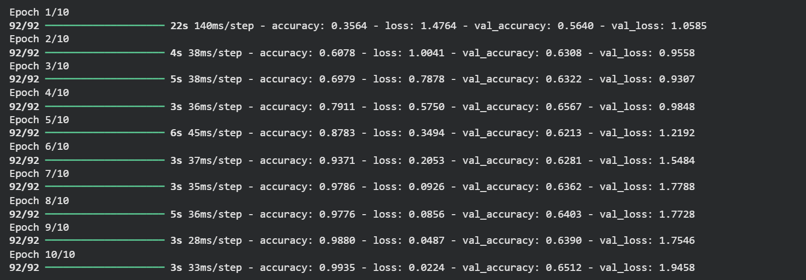Training output showing 99%+ training accuracy

99.35% training accuracy. 🎉

...but wait. Look at the validation accuracy. It's sitting around 65%. That's a red flag.

---

The Overfitting Problem

Let's plot the training curves to really see what's going on.

acc = history.history['accuracy']
val_acc = history.history['val_accuracy']
loss = history.history['loss']
val_loss = history.history['val_loss']

epoch_range = range(epochs)

plt.figure(figsize=(8, 8))
plt.subplot(1, 2, 1)
plt.plot(epoch_range, acc, label='Training Accuracy')
plt.plot(epoch_range, val_acc, label='Validation Accuracy')
plt.legend(loc='lower right')
plt.title('Training and Validation Accuracy')

plt.subplot(1, 2, 2)
plt.plot(epoch_range, loss, label='Training Loss')
plt.plot(epoch_range, val_loss, label='Validation Loss')
plt.legend(loc='upper right')
plt.title('Training and Validation Loss')
plt.show()

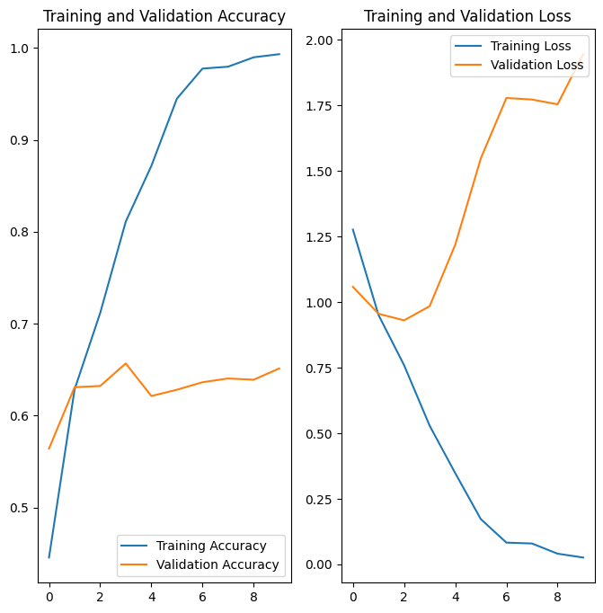Training vs validation accuracy/loss curves showing classic overfitting

Yep — classic overfitting. You can see it clearly:

• Training accuracy climbs smoothly toward 100%
• Validation accuracy plateaus early, hovering around 60%
• The gap between the two curves keeps growing

What's happening? The model has basically memorized the training images — including all their noise, weird lighting, and quirks. When it sees a new flower image it's never encountered before, it doesn't know what to do with it.

The root cause is that our dataset is relatively small. With limited data, there aren't enough examples for the model to learn truly general patterns. It cheats by memorizing instead.

---

Fixing Overfitting: Data Augmentation + Dropout

We're going to tackle this from two angles.

Data Augmentation creates new training examples on-the-fly by randomly transforming existing images — flipping them, rotating them slightly, zooming in a bit. The model sees a "different" version of the image each epoch, which forces it to learn features that are robust to these variations rather than memorizing exact pixel patterns.

Dropout randomly disables a fraction of neurons during training (we'll use 20%). This stops neurons from over-relying on specific other neurons, which is a huge source of overfitting. The model is forced to learn redundant, distributed representations of features — which generalize much better.

One important thing to know: dropout only applies during training. At inference time, all neurons are active, but Keras scales down the weights proportionally to compensate. So your predictions remain consistent.

Here's the updated model:

data_augmentation = keras.Sequential([
    layers.RandomFlip("horizontal", input_shape=(img_height, img_width, 3)),
    layers.RandomRotation(0.1),
    layers.RandomZoom(0.1),
])

model = Sequential([
    data_augmentation,
    layers.Rescaling(1./255),
    layers.Conv2D(16, 3, padding='same', activation='relu'),
    layers.MaxPooling2D(),
    layers.Conv2D(32, 3, padding='same', activation='relu'),
    layers.MaxPooling2D(),
    layers.Conv2D(64, 3, padding='same', activation='relu'),
    layers.MaxPooling2D(),
    layers.Dropout(0.2),
    layers.Flatten(),
    layers.Dense(128, activation='relu'),
    layers.Dense(num_classes)
])

Compile and train with the same code as before, then look at those curves again:

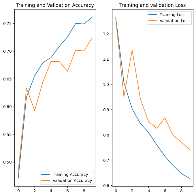Curve after removing overfitting

72.34% validation accuracy — and more importantly, the training and validation curves are moving together now. The model is actually generalizing.

Could we push the accuracy higher? Absolutely. Running for more epochs would help. You could also explore transfer learning (using a pretrained model like MobileNet), tuning the learning rate, or adding more augmentation. But for a from-scratch CNN on a small dataset, 72% is a solid baseline.

---

Running Inference

Let's make sure the model actually works before we ship it. We'll download a sunflower image and see what it predicts.

sunflower_url = "https://storage.googleapis.com/download.tensorflow.org/example_images/592px-Red_sunflower.jpg"
sunflower_path = tf.keras.utils.get_file('Red_sunflower', origin=sunflower_url)

img = tf.keras.utils.load_img(
    sunflower_path, target_size=(img_height, img_width)
)

img_array = tf.keras.utils.img_to_array(img)
img_array = tf.expand_dims(img_array, 0)  # add batch dimension

predictions = model.predict(img_array)
score = tf.nn.softmax(predictions[0])

print(
    "This image most likely belongs to {} with a {:.2f}% confidence."
    .format(class_names[np.argmax(score)], 100 * np.max(score))
)

Since the output layer gives us raw logits (not probabilities), we apply tf.nn.softmax to convert them into a probability distribution across all classes. Then np.argmax picks the class with the highest probability.

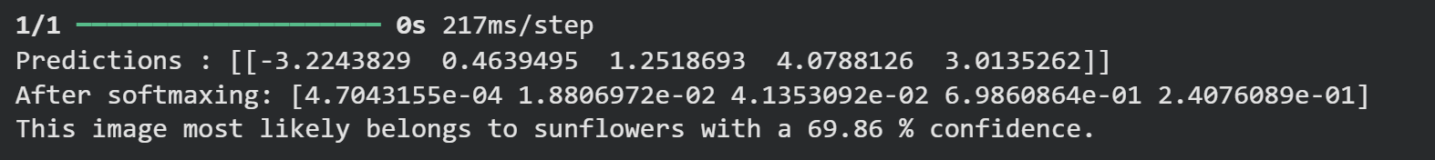Inference output correctly predicting sunflower

It correctly identified the sunflower.

---

Converting to TFLite for Mobile

Running a full Keras model on a phone would be painfully slow and memory-hungry. TensorFlow Lite is a trimmed-down version of TensorFlow optimized for mobile and edge devices — it quantizes and compresses the model so it can run efficiently on constrained hardware.

Converting is surprisingly easy:

converter = tf.lite.TFLiteConverter.from_keras_model(model)
tflite_model = converter.convert()

with open('model.tflite', 'wb') as f:
    f.write(tflite_model)

That's it. Your model is now a binary .tflite file, ready to be bundled into a mobile app.

Let's verify it works by loading it back and running inference through the TFLite interpreter:

TF_MODEL_FILE_PATH = 'model.tflite'

interpreter = tf.lite.Interpreter(model_path=TF_MODEL_FILE_PATH)

# Check the model's input/output signature
print(interpreter.get_signature_list())

Signature list showing serving_default with keras_tensor_15 input and output_0

The model exposes a serving_default signature. The input tensor is named keras_tensor_15 and the output is output_0. We use these names to invoke the model:

classify_lite = interpreter.get_signature_runner('serving_default')

prediction_lite = classify_lite(keras_tensor_15=img_array)['output_0']
score_lite = tf.nn.softmax(prediction_lite)

print(
    "This image most likely belongs to {} with a {:.2f}% confidence."
    .format(class_names[np.argmax(score_lite)], 100 * np.max(score_lite))
)

TFLite inference output matching the original model prediction

Same result as the full Keras model — perfect. The TFLite conversion didn't degrade the output at all.

---

Wrapping Up

Here's what we did today:

• Built a baseline CNN and saw it overfit hard
• Fixed overfitting with data augmentation and dropout, jumping from ~65% to ~72% validation accuracy
• Ran inference and confirmed the model works
• Converted the model to .tflite format for mobile deployment

In Part 3, we're going to take this model.tflite file and build an actual Flutter app around it — one that lets you point your camera at a flower and classify it on-device, with zero internet connection needed. If that sounds cool to you, subscribe to the newsletter below and I'll drop it straight in your inbox the moment it's live.

Thanks for reading. Keep building. 🚀