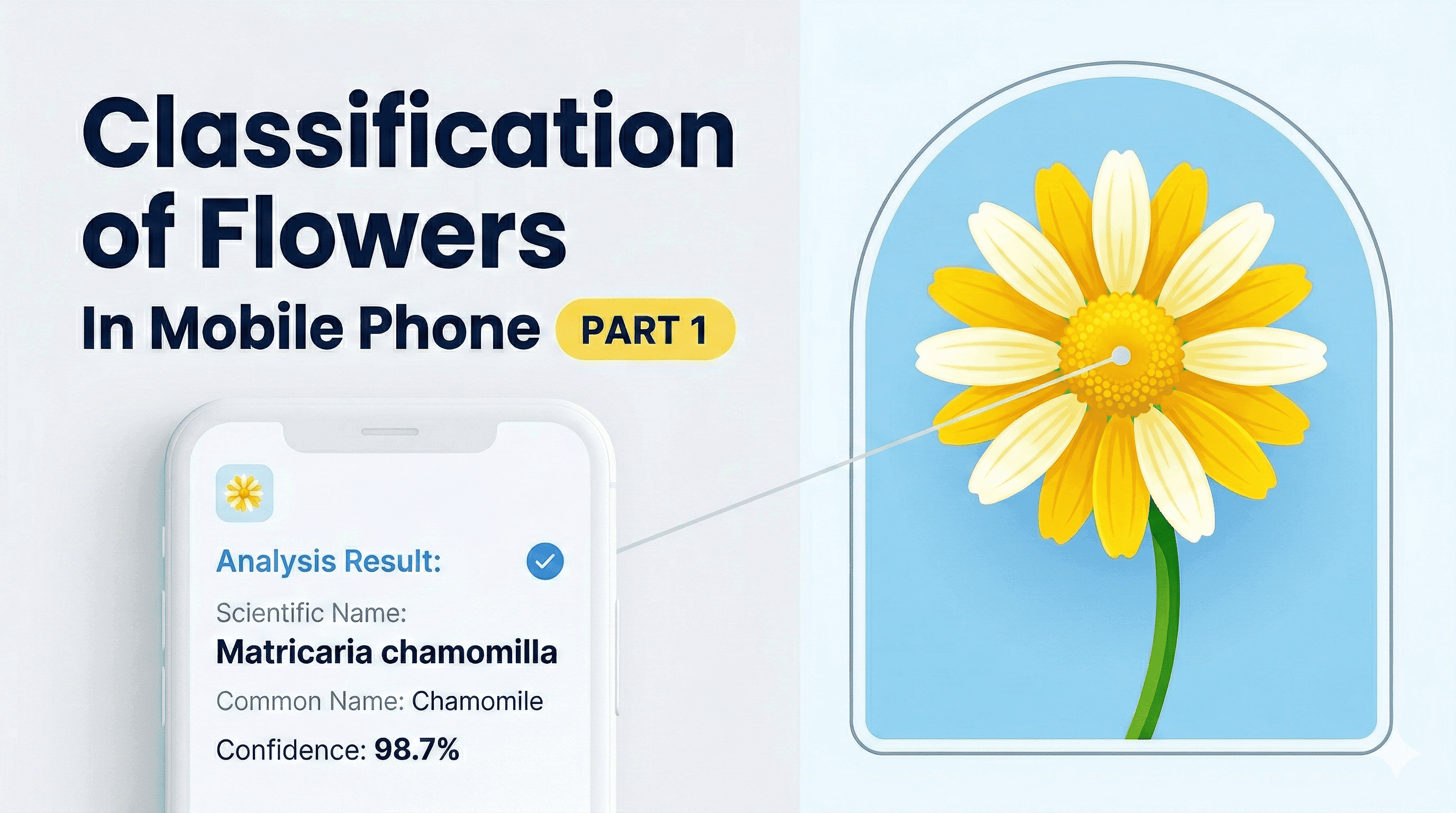
Classification of Flowers In Mobile Phone ( PART 1)

Hey, welcome! 👋

I've always been fascinated by the idea of a world where powerful AI runs entirely on your device — no cloud, no internet dependency, no latency. Just pure on-device intelligence.

That future is closer than you think, and edge computing is leading the charge. It's one of the most exciting areas in AI right now, and honestly one of the most meaningful — because getting capable models running locally is how we bring these tools to people who don't have reliable internet access.

So here's what we're building: a Flutter app that classifies flowers on your Android phone, entirely offline. No API calls. No cloud model. Just a .tflite file sitting on your device doing its thing.

We're splitting this into three parts:

• Part 1 (this one) — Load the dataset, build a clean data pipeline, and prep everything for training
• Part 2 — Train a CNN, fix overfitting, and convert the model to TFLite
• Part 3 — Build the Flutter app and deploy the model on-device

Alright, let's get into it. Buckle up.

---

1. Importing the Libraries

import pathlib
import matplotlib.pyplot as plt
import numpy as np
import PIL
import tensorflow as tf
from tensorflow import keras
from tensorflow.keras import layers
from tensorflow.keras.models import Sequential

Nothing surprising here — we've got our image handling, visualization, and Keras all imported. This is our full toolkit for the data pipeline we're about to build.

---

2. Downloading and Exploring the Dataset

We need thousands of flower images to train on. Thankfully, Google hosts a great example dataset for exactly this kind of thing. The dataset comes compressed as a .tgz tarball, so we need to download and extract it.

tf.keras.utils.get_file handles the whole thing in one line:

dataset_url = "https://storage.googleapis.com/download.tensorflow.org/example_images/flower_photos.tgz"
data_dir = tf.keras.utils.get_file('flower_photos.tar', origin=dataset_url, extract=True)
data_dir = pathlib.Path(data_dir).with_suffix('')  # strip the .tar extension
data_dir = data_dir / 'flower_photos'              # the actual images live in this subdirectory

This one call does a lot of heavy lifting: it fetches the file from the URL, saves it locally, caches it so we don't re-download on subsequent runs, and with extract=True, decompresses the archive automatically. Then we use pathlib.Path to get a nice path object we can work with cleanly.

Let's peek at what's inside:

for item in data_dir.glob("*"):
    print(item.name)

LICENSE.txt
roses
daisy
sunflowers
dandelion
tulips

Each flower species has its own folder. This folder structure is exactly what we need — we'll use the folder names as class labels.

class_names = np.array(sorted([
    item.name for item in data_dir.glob('*')
    if item.name != "LICENSE.txt"
]))
print(class_names)
# ['daisy' 'dandelion' 'roses' 'sunflowers' 'tulips']

And how many images do we have total?

image_count = len(list(data_dir.glob('*/*.jpg')))
print(image_count)  # 3670 images

3,670 images across 5 classes. Not huge, but workable — especially once we add data augmentation in Part 2.

---

3. Building the Data Pipeline

This is where things get interesting. We're going to build a custom tf.data pipeline from scratch, which gives us full control over how the data flows into the model.

Step 1: List all image paths (without shuffling yet)

list_ds = tf.data.Dataset.list_files(str(data_dir / '*/*'), shuffle=False)

This creates a dataset of file paths — just the paths, not the actual images. We deliberately skip shuffling here so we can do it ourselves with more control in the next step.

Step 2: Shuffle with a fixed seed

list_ds = list_ds.shuffle(buffer_size=image_count, reshuffle_each_iteration=False)

reshuffle_each_iteration=False is important — it means the order stays the same across epochs. This matters for the train/validation split we're about to do: if the order changed every run, our splits would bleed into each other.

Step 3: Split into train and validation sets

We'll use an 80/20 split — 20% for validation, the rest for training.

val_size = int(image_count * 0.2)
train_ds = list_ds.skip(val_size)  # 2936 images
val_ds = list_ds.take(val_size)    # 734 images

Step 4: Load and decode the images

Right now our dataset only holds file paths. We need to actually read and decode each image from disk. There are two things we need to handle:

1. Images on disk are compressed (JPEG). We need to decode them into raw RGB pixel arrays.
2. Images come in all sorts of sizes. We need to resize them to a consistent 180×180 so every input to the model is the same shape.

We also need to extract the label from the file path. Since each image lives in a folder named after its class (like flowers_data/roses/image.jpg), we can grab the second-to-last part of the path and match it against our class names.

AUTOTUNE = tf.data.AUTOTUNE
img_height = 180
img_width = 180

def get_label(file_path):
    parts = tf.strings.split(file_path, '/')
    one_hot = parts[-2] == class_names  # [False, False, True, False, False] for 'roses'
    return tf.argmax(one_hot)           # returns the integer index of the class

def decode_img(img):
    img = tf.image.decode_jpeg(img, channels=3)          # decompress to RGB
    return tf.image.resize(img, [img_height, img_width]) # resize to 180x180

def process_path(file_path):
    label = get_label(file_path)
    img = tf.io.read_file(file_path)  # read raw bytes from disk
    img = decode_img(img)
    return img, label

train_ds = train_ds.map(process_path, num_parallel_calls=AUTOTUNE)
val_ds = val_ds.map(process_path, num_parallel_calls=AUTOTUNE)

The num_parallel_calls=AUTOTUNE part is key for performance — it tells TensorFlow to process multiple file paths in parallel, using however many CPU threads make sense for your hardware. This keeps your CPU/GPU busy instead of waiting on disk reads one at a time.

Let's do a quick sanity check to make sure the pipeline is working:

for image, label in train_ds.take(2):
    print("Image shape:", image.numpy().shape)
    print("Label:", label)

Output showing image shape (180, 180, 3) and integer label

Each image comes out as a (180, 180, 3) tensor with an integer label.

---

4. Configuring the Dataset for Performance

We have a working pipeline — but "working" and "fast" are two different things. Before we hand this dataset off to the model, we need to configure it so the data loading never becomes a bottleneck during training.

The two techniques that matter most here:

Prefetching — While the model is training on batch t, the pipeline starts preparing batch t+1 in the background. By the time the model is done with the current batch and asks for the next one, it's already ready. This overlap is huge for GPU utilization.

Caching — On the first epoch, images are read from disk and decoded. Caching saves the processed tensors in memory, so every subsequent epoch reads from RAM instead of disk. Much faster.

def configure_dataset_for_performance(ds):
    ds = ds.cache()                          # cache after first epoch
    ds = ds.shuffle(buffer_size=1000)        # shuffle within each epoch
    ds = ds.batch(32)                        # group into batches of 32
    ds = ds.prefetch(buffer_size=AUTOTUNE)   # prepare next batch in the background
    return ds

train_ds = configure_dataset_for_performance(train_ds)
val_ds = configure_dataset_for_performance(val_ds)

Let's visualize a batch to make sure everything looks right:

image_batch, label_batch = next(iter(train_ds))

plt.figure(figsize=(10, 10))
for i in range(9):
    ax = plt.subplot(3, 3, i + 1)
    plt.imshow(image_batch[i].numpy().astype("uint8"))
    plt.title(class_names[label_batch[i]])
    plt.axis("off")

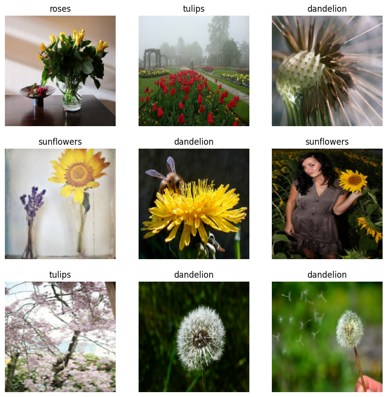Grid of 9 flower images with correct labels

Different flower types, randomly mixed, correctly labeled. The pipeline is working exactly as expected.

---

5. A Note on Pixel Rescaling

One last thing before we wrap up. You'll notice the images currently have pixel values ranging from 0 to 255. Neural networks don't love large input values — they tend to learn faster and more stably when inputs are small, ideally in the [0, 1] range.

Rather than rescaling here in the pipeline, we're going to handle it inside the model itself using a Rescaling layer. Doing it this way means the transformation is baked into the model — so when we deploy the .tflite file and run inference on new images, we don't need to remember to rescale inputs manually. The model just handles it. Cleaner for deployment.

We'll set that up in Part 2.

---

That's a wrap for Part 1! We went from a raw URL to a fully optimized tf.data pipeline with batching, caching, prefetching, and parallel processing. The groundwork is solid.

In Part 2, we'll build and train a CNN on this dataset, tackle overfitting head-on, and convert the final model to .tflite format. If you want a heads-up when it drops, subscribe to the newsletter below — I'll send it straight to your inbox.

See you in Part 2. Happy coding!